Review of linear regression (skip to horizontal line for new stuff)
Least squares linear regression
In matlab this can be solved for with the \ operator
A\B is the matrix division of A into B, which is roughly the
same as INV(A)*B , except it is computed in a different way.
If A is an N-by-N matrix and B is a column vector with N
components, or a matrix with several such columns, then
X = A\B is the solution to the equation A*X = B computed by
Gaussian elimination.
mb= [1 1; 3 1]\[2;4] (left matrix divide)
What if a line is not a good fit?
The linear regression technique
can easily be extended to non-linear regression by adding in
non-linear terms
Let's say you want to fit
y=mx + nx^2 + b
How do we solve this, well if we precompute x^2 for our data
we have the following problem.
2 =m(1) + n(1) + b
4 =m(3) + n(9) + b
3.5 =m(2) + n(4) + b
We can write this in matrix form
[2 ; 4; 3.5] = [ 1 1 1; 3 9 1; 2 4 1] *[m; n; b]
A=[1 1 1; 3 9 1; 2 4 1]
y= [ 2; 4; 3.5]
Again we can solve this with
mnb= A\y
Let's plot this on our graph
In order to plot this curve we will simply compute values
for many x points and join them with lines
xp=0:.1:5;
yp=mnb(1)*xp+mnb(2)*xp.^2 + mnb(3);
plot(xp,yp,'g')
Now let's consider a larger dataset
x=0:6
y=x.^2 + 3*randn(1,length(x))
plot(x,y,'*')
A = [ x' ones(length(x),1)]
mb= A\y'
xp=0:.1:6
yp=mb(1)*xp +mb(2)
hold on
plot(xp,yp)
A = [ x' x.^2' ones(length(x),1)]
mnb=A\y'
xp=0:.1:6
yp=mnb(1)*xp +mnb(2)*xp.^2+ mnb(3)
plot(xp,yp,'r')
%This is a better fit. What if we take this further
%Here we try to fit
%y=mx + nx^2 +px^3 + b
A = [ x' x.^2' x.^3' ones(length(x),1)]
mnpb=A\y'
xp=0:.1:6
yp=mnpb(1)*xp +mnpb(2)*xp.^2+ mnpb(3)*xp.^3 + mnpb(4)
plot(xp,yp,'g')
%How about
%y=mx+nx^2 +px^3 + qx^4 + rx^5+b
A = [ x' x.^2' x.^3' x.^4' x.^5' ones(length(x),1)]
mnpqrb=A\y'
xp=0:.1:6
yp=mnpqrb(1)*xp +mnpqrb(2)*xp.^2+ mnpqrb(3)*xp.^3 + mnpqrb(4)*xp.^4 + mnpqrb(5)*xp.^5 + mnpqrb(6)
plot(xp,yp,'k')
% Which fit looks best to you?
% How can a machine learning system recognize this?
% We refer to the problem shown by the black line as OVERFITING
% One useful technique is to leave out some datapoints and look at how
% well the resulting curve fits those datapoints
x=0:6
y=x.^2 + 3*randn(1,length(x))
clf
plot(x,y,'*')
hold on
totsqerr=0
totsqerr2=0
for i=1:7 % leave out each datapoint in turn
if i==1
xuse=x(2:7)
yuse=y(2:7)
elseif i==7
xuse=x(1:6)
yuse=y(1:6)
else
xuse=x([1:i-1, i+1:7])
yuse=y([1:i-1, i+1:7])
end
xleftout=x(i);
A = [ xuse' xuse.^2' xuse.^3' xuse.^4' xuse.^5' ones(length(xuse),1)];
mnpqrb=A\yuse';
mnb=A(:,[1:2 6])\yuse';
xp=0:.1:6;
yp=mnpqrb(1)*xp +mnpqrb(2)*xp.^2+ mnpqrb(3)*xp.^3 + mnpqrb(4)*xp.^4 + mnpqrb(5)*xp.^5 + mnpqrb(6);
plot(xp,yp,'k')
yp2=mnb(1)*xp + mnb(2)*xp.^2 +mnb(3);
plot(xp,yp2,'r')
%%compute yleftout
yleftout= predyval(xleftout,mnpqrb);
yleftout2= predyval(xleftout,mnb);
%%% compute squared error for left out point
sqerr=(yleftout-y(i))^2
sqerr2=(yleftout2-y(i))^2
totsqerr=sqerr+totsqerr;
totsqerr2=sqerr2+totsqerr2;
end
rootmeansqerr=sqrt(totsqerr/7)
rootmeansqerr2=sqrt(totsqerr2/7)
So we were able to do interesting non-linear fitting in the above
case because the fit was linear in the parameters (m,n,p,q,r,b).
There will be many cases where you want something more general and
the fit will be non-linear in the parameters.
e.g.
1) y=a sin(b x) This is linear in a but not b
2) y=c e^(-dx) + e linear in c and e but not d
What can we do in this case?
We can no longer do a "closed-form" solution, but must use iterative techniques.
The big picture is you want to optimize some function
(e.g. 1/N \sum_i (y(i)-f(x_i))^2 ) mean sum square error
or take the square root of the above = root mean square error
you can consider an "error surface" which is a function of the parameters
(e.g. a,b in Equation 1) a few lines above) For different values of a and
b , different values of y as a function of x will be predicted. One can compute the mean sum square error for each a,b over the dataset. This would give a surface as a function of a,b. Ideally we'd like to find the minimum on that surface. But we can't see that surface, all we can do is sample from that surface
(with a computation) and later we'll see where we can sample values and derivatives. For now we look at one solution which just samples values.
One solution in matlab is to use the fminsearch function
which uses the Nelder-Mead (Simplex) Method for function fitting
see
How does fminsearch work?
http://www.boomer.org/c/p3/c11/c1106.html
http://www.scholarpedia.org/article/Nelder-Mead_algorithm
(Note notation not consistent with applet below (beta and gamma are reversed between the scholarpedia page and the applet page below)
http://www.cse.uiuc.edu/iem/optimization/NelderMead/
Info on Matlab's implementation
The method works with a number of rules. The starting point is used to construct a simplex, a shape with m+1 points, where m is the number of parameters. (Note that m+1 points is the smallest number of points to enclose a volume in dimensionality m)
Thus for a two parameter problem there are three points, a triangle. The program calculates the
Function evaluation at each point of the simplex on the Function surface (e.g. summed square error SSE).
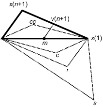
The Rules (see figure below also)
* Reflect the point with the highest SSE (x(n+1) in figure below) through centroid (center) of the simplex (using alpha) (this gives r in figure below)
* If this is just a good point (intermediate between other SSE values) accept the reflected point as the new simplex point and terminate this iteration.
* If this produces the new lowest SSE (best point) test a point that expands the simplex further (using beta - s in the figure below) -- if this point is worse than the original reflected point, accept the original reflected point (r), otherwise accept the new expanded point (s). In either case terminate this iteration.
* If this is the highest SSE (worst point) test a point that contracts the simplex and reflects closer (using gamma)
* * For contraction, if the new point (r) is worse than the old point that is being reflected (x(n+1)) then contract back from the old point (contract back to cc), otherwise contract back from the new point (contract back to c).
* * If the new contracted point (c or cc) is worse than the reflected point (r) , undo the whole step (from reflection) and do shrink operation instead
* * * In the shrink operation all but the best SSE points are brought down towards the best (lowest SSE) point. (e.g. x(n+1) moves to v(n+1) in the figure - each of the other points other than x(1) also moves towards x(1)) Terminate this iteration
These rules are repeated until the convergence criteria are meet. The simplex moves over WSS surface and should contract around minimum.
alpha - gives how far to reflect beyond the simplex (1 gives full reflection)
beta - how far to expand by (2 says go twice as far past the simplex)
gamma - how far to contract by (0 says contract back to simplex edge, 1 says don't contract at all - (use old point if it was better otherwise use new point)) If it is worse than before then contract back from old point, otherwise contract back from new point.
Here is the figure from the Matlab page Info on Matlab's implementation
showing the different possibilities where x(n+1) was the worst point, x(1) the best point. r is the originally
reflected point. s is the expansion considered point (when c is better than x(1)). c is the contraction considered point when
r is worse than x(n) but better than x(n+1). cc is the contraction considered point when r is worse than x(n+1). v(n+1) is the
shrunk point of x(n+1) when cc or c are worse than r.
Fminsearch uses the simplex search method of [1]. This is a direct
search method that does not use numerical or analytic gradients. If n
is the length of x, a simplex in n-dimensional space is characterized
by the n+1 distinct vectors that are its vertices. In two-space, a
simplex is a triangle; in three-space, it is a pyramid. At each step
of the search, a new point in or near the current simplex is
generated. The function value at the new point is compared with the
function's values at the vertices of the simplex and, usually, one of
the vertices is replaced by the new point, giving a new simplex. This
step is repeated until the diameter of the simplex is less than the
specified tolerance
[1] Lagarias, J.C., J. A. Reeds, M. H. Wright, and P. E. Wright, "Convergence Properties of the Nelder-Mead Simplex Method in Low Dimensions," SIAM Journal of Optimization, Vol. 9 Number 1, pp. 112-147, 1998.
FMINSEARCH Multidimensional unconstrained nonlinear minimization (Nelder-Mead).
X = FMINSEARCH(FUN,X0) starts at X0 and attempts to find a local minimizer
X of the function FUN. FUN accepts input X and returns a scalar function
value F evaluated at X. X0 can be a scalar, vector or matrix.
----------------------------------------------------------
How is fminsearch (that finds a minimum of a function)
used to fit a nonlinear function.
We use fminsearch to find the minimum of the
mean square error between the current fit and the target values
In the example below we will be fitting the function
f(x)=ax+bx^2 + c exp(-dx) + e
by finding the best a,b,c,d,e to fit the given x, y data
We could use the simplex search method to find all the parameters
(linear and non-linear) but it is better (faster and less dependent on
initial conditions) to use our old linear regression
technique to fit the linear parameters for a given non-linear parameter version.
In the code below we have done it both ways. The slow way
(using the simplex code for finding all parameters)
in myfitfunslow.m and myfitdemoslow.m
And the fast way, using only fminsearch(simplex method) for finding
the nonlinear parameter d and linear regression to find the linear
parameters a,b,c,e.
This more efficient method is in code
my fitdemo.m and myfitfun.m
--------------------------------------------------------------------------
%% Optimal Fit of a Non-linear Function
% This is a demonstration of the optimal fitting of a non-linear function to a
% set of data. It uses FMINSEARCH, an implementation of the Nelder-Mead simplex% (direct search) algorithm, to minimize a nonlinear function of several
% variables.
%
% Modified by VdS from program fitdemo by
% Copyright 1984-2004 The MathWorks, Inc.
% $Revision: 5.15.4.2 $ $Date: 2004/08/16 01:37:29 $
%%
% First, create some sample data and plot it.
x = (0:.1:2)';
y = [5.8955 3.5639 2.5173 1.9790 1.8990 1.3938 1.1359 1.0096 1.0343 ...
0.8435 0.6856 0.6100 0.5392 0.3946 0.3903 0.5474 0.3459 0.1370 ...
0.2211 0.1704 0.2636]';
plot(x,y,'ro'); hold on; h = plot(x,y,'b'); hold off;
title('Input data'); ylim([0 6])
%%
% The goal is to fit the following function with three linear parameters and one
% nonlinear parameter to the data:
%
% y = ax + bx^2 + c*exp(-d*x) + e
%
% To fit this function, we've create a function MYFITFUN. Given the nonlinear
% parameter (lambda) and the data (x and y), FITFUN calculates the error in the
% fit for this equation and updates the line (h).
type myfitfunslow
%%
% Make a guess for initial estimate of a b c d and e (start)
% and invoke FMINSEARCH. It
% minimizes the error returned from MYFITFUN by adjusting them. It returns the
% final values of a b c d and e.
start = [-2; 1; 4; 1; 2];
options = optimset('TolX',0.1); % termination tolerance on x
%% fminsearch will perform the Nelder-Mead algorithm for parameter vector x
%% using myfitfunslow to compute the error values
estimated_abcde = fminsearch(@(abcde) myfitfunslow(abcde,x,y,h),start,options)
--------------------------------------------------------------------
function err = myfitfunslow(abcde,x,y,handle)
%FITFUN Used by FITDEMO.
% FITFUN(lambda,t,y,handle) returns the error between the data and the values
% computed by the current function of lambda.
%
% modified by VdS from
% Copyright 1984-2002 The MathWorks, Inc.
% $Revision: 5.8 $ $Date: 2002/04/15 03:36:42 $
% evaluate the function with the given parameters at the given data points (x)
z= abcde(1)*x+abcde(2)*x.^2 + abcde(3)*exp(-abcde(4)*x) + ones(length(x),1)*abcde(5);
% compute the error from the supplied ys
err = norm(z-y);
set(gcf,'DoubleBuffer','on');
set(handle,'ydata',z)
drawnow
pause(.04)
------------------------------------------------------------------
%% Optimal Fit of a Non-linear Function
% This is a demonstration of the optimal fitting of a non-linear function to a
% set of data. It uses FMINSEARCH, an implementation of the Nelder-Mead simplex% (direct search) algorithm, to minimize a nonlinear function of several
% variables.
%
% Modified by VdS from program fitdemo by
% Copyright 1984-2004 The MathWorks, Inc.
% $Revision: 5.15.4.2 $ $Date: 2004/08/16 01:37:29 $
%%
% First, create some sample data and plot it.
x = (0:.1:2)';
y = [5.8955 3.5639 2.5173 1.9790 1.8990 1.3938 1.1359 1.0096 1.0343 ...
0.8435 0.6856 0.6100 0.5392 0.3946 0.3903 0.5474 0.3459 0.1370 ...
0.2211 0.1704 0.2636]';
plot(x,y,'ro'); hold on; h = plot(x,y,'b'); hold off;
title('Input data'); ylim([0 6])
%%
% The goal is to fit the following function with three linear parameters and one
% nonlinear parameter to the data:
%
% y = ax + bx^2 + c*exp(-d*x) + e
%
% To fit this function, we've create a function MYFITFUN. Given the nonlinear
% parameter (lambda) and the data (x and y), FITFUN calculates the error in the
% fit for this equation and updates the line (h).
type myfitfun
%%
% Make a guess for initial estimate of d (start) and invoke FMINSEARCH. It
% minimizes the error returned from MYFITFUN by adjusting d. It returns the
% final value of d. Within MYFITFUN optimal values for a,b,c and e for
% the current d are found.
start = [1];
options = optimset('TolX',0.1); % termination tolerance on x
estimated_d = fminsearch(@(d) myfitfun(d,x,y,h),start,options)
-----------------------------------------------------------
function err = myfitfun(d,x,y,handle)
%FITFUN Used by FITDEMO.
% FITFUN(lambda,t,y,handle) returns the error between the data and the values
% computed by the current function of lambda.
%
% modified by VdS from
% Copyright 1984-2002 The MathWorks, Inc.
% $Revision: 5.8 $ $Date: 2002/04/15 03:36:42 $
A = [x x.^2 exp(-d*x) ones(length(x),1)];
abce = A\y
z = A*abce;
err = norm(z-y);
set(gcf,'DoubleBuffer','on');
set(handle,'ydata',z)
drawnow
pause(.04)